The long-range properties of a weakly interacting one-dimensional bosonic gas can be
calculated using the macroscopic representation of the field operator (1.1):
![]() , where
, where
![]() is the mean density1.16 and
is the mean density1.16 and
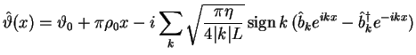
![]() is the phase
operator. Those operators can be expressed in terms of quasiparticle creation and
annihilation operators (see., for example, [PS03] Eqs.(6.65-6.66), and
consider a one-dimensional system):
is the phase
operator. Those operators can be expressed in terms of quasiparticle creation and
annihilation operators (see., for example, [PS03] Eqs.(6.65-6.66), and
consider a one-dimensional system):
The operators (1.155,1.156) satisfy the commutation rule
![]() .
.
Our approach is applicable in a weakly interacting gas
![]() . Deep in this
regime the speed of sound has a square root dependence on the density
. Deep in this
regime the speed of sound has a square root dependence on the density
![]() and the coefficient
and the coefficient ![]() is large
is large
![]() . In the opposite regime of strong correlations
. In the opposite regime of strong correlations ![]() (TG limit) the bosonic system of impenetrable particles is mapped onto a system
of non-interacting fermions [Gir60] with the speed of sound given by the
fermi velocity
(TG limit) the bosonic system of impenetrable particles is mapped onto a system
of non-interacting fermions [Gir60] with the speed of sound given by the
fermi velocity
![]() (1.100) and is proportional to the
density. In this regime
(1.100) and is proportional to the
density. In this regime ![]() . By generalizing the definition of the fermi
velocity from the TG regime, where the fermionization of a bosonic system happens,
to an arbitary density we obtain a simple interpretation of the parameter
(1.157):
. By generalizing the definition of the fermi
velocity from the TG regime, where the fermionization of a bosonic system happens,
to an arbitary density we obtain a simple interpretation of the parameter
(1.157): ![]() . The speed of sound in a system with a repulsive
contact potential is not larger than the fermi velocity, thus in LL system
(5.1)
. The speed of sound in a system with a repulsive
contact potential is not larger than the fermi velocity, thus in LL system
(5.1) ![]() . The situation becomes different in a gas of hard-rods of
size
. The situation becomes different in a gas of hard-rods of
size ![]() . Presence of an excluded volume makes the available phase space be
effectively smaller
. Presence of an excluded volume makes the available phase space be
effectively smaller
![]() , which in turn renormalizes the speed of sound (see
1.103) and makes it be larger. In this special case of the super-Tonks gas (Sec. 6) the parameter
, which in turn renormalizes the speed of sound (see
1.103) and makes it be larger. In this special case of the super-Tonks gas (Sec. 6) the parameter
![]() (1.157) can be smaller than
(1.157) can be smaller than ![]() .
.
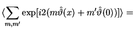
Following Haldane [Hal81] we introduce a new field
![]() such
that
such
that
![]() .
The operator
.
The operator ![]() satisfy boundary conditions
satisfy boundary conditions
![]() and increases monotonically by
and increases monotonically by ![]() each
time
each
time ![]() passes the location of a particle. Particles are thus taken to be located
at the points where
passes the location of a particle. Particles are thus taken to be located
at the points where
![]() is a multiple of
is a multiple of ![]() , allowing the density
operator to be expressed as
, allowing the density
operator to be expressed as
![]() , or, equivalently,
, or, equivalently,
![$\displaystyle \hat\rho(x) = [\rho_0 + \hat\rho^{\prime}(x)] \sum\limits_{m=-\infty}^\infty
\exp[i2m\hat\vartheta(x)]$](img613.gif) |
(1.158) |
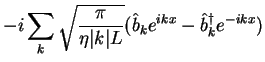
Integrating (1.156) we obtain an expression of this field in terms of creation
and annihilation operators:
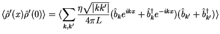
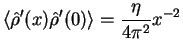
We will start with calculation of asymptotics of the density-density correlation
function:
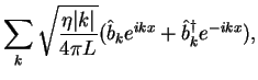
First of all we calculate the contribution coming from density fluctuations
![]() :
:
The creation and annihilation operators satisfy bosonic commutation relations
![]() and at
zero temperature excitations are absent
and at
zero temperature excitations are absent
![]() , so in the averaging in Eq. 1.161 we get non
zero result only for
, so in the averaging in Eq. 1.161 we get non
zero result only for
![]() , i.e.
, i.e.
 |
(1.162) |
We consider contribution only from the lower limit of the integration ![]() and, thus, obtain
and, thus, obtain
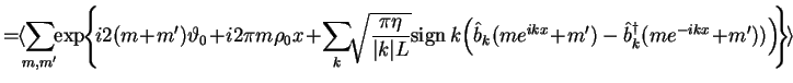
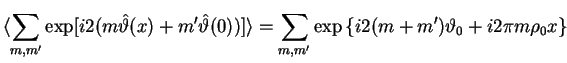
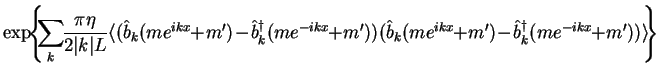
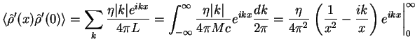
Now let us calculate the contribution of the phase fluctuations in (1.160):
An average of a phonon operator ![]() is gaussian and satisfy
an equality
is gaussian and satisfy
an equality
![]() . In
this way we can pass from an average of an exponent to an exponent of averaged
quantities:
. In
this way we can pass from an average of an exponent to an exponent of averaged
quantities:
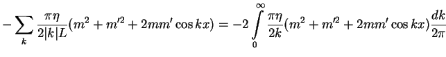
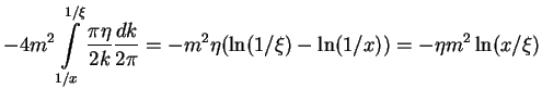
At the zero temperature excitations are absent. This simplifies the calculation as
the averaging in (1.165) gives simply
![]() . We substitute the summation in the exponent
of (1.165) with integration over
. We substitute the summation in the exponent
of (1.165) with integration over ![]() :
:
This integral has an infrared divergence unless
![]() , so we consider
only these terms. Now the integral converges at small
, so we consider
only these terms. Now the integral converges at small ![]() and takes the leading
contribution in the interval
and takes the leading
contribution in the interval ![]() where
where ![]() is minimal length at which
the hydrodinamic theory can be applied. In this region one can neglect the
contribution coming from the oscillating cosine term and one has
is minimal length at which
the hydrodinamic theory can be applied. In this region one can neglect the
contribution coming from the oscillating cosine term and one has
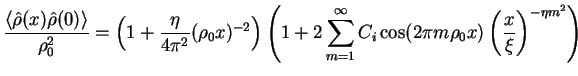
Finally, collecting together (1.163,1.164,1.167) we obtain
an expression for the stationary density-density correlation function

![$\displaystyle \langle\hat\rho(x)\hat\rho(0)\rangle \approx
(\rho_0^2 + \langle\...
...ts_{m,m^{\prime}}
\exp[i2(m\hat\vartheta(x)+m^{\prime}\hat\vartheta(0))]\rangle$](img615.gif)