For tightly-confined trapped gases the 1D regime is reached if the transverse
motion of the atoms is frozen, with all the particles occupying the ground state of
the transverse harmonic oscillator. At zero temperature, this condition requires
that the energy per particle is dominated by the trapping potential,
![]() , where the excess energy
, where the excess energy ![]() is much
smaller than the separation between levels in the transverse direction,
is much
smaller than the separation between levels in the transverse direction,
![]() . In the following we consider situations where the
Bose gas is in the 1D regime for any value of the 3D scattering length
. In the following we consider situations where the
Bose gas is in the 1D regime for any value of the 3D scattering length ![]() .
For a fixed trap anisotropy parameter
.
For a fixed trap anisotropy parameter ![]() and a fixed number of particles
and a fixed number of particles ![]() the above requirement is satisfied if
the above requirement is satisfied if ![]() . For
. For ![]() and
and
![]() (as considered in Sec. 4.4.1) this condition is fulfilled.
(as considered in Sec. 4.4.1) this condition is fulfilled.
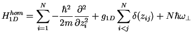
To compare the 3D and 1D energetics of a Bose gas, we consider the 3D and 1D
Hamiltonian describing ![]() spin-polarized bosons,
spin-polarized bosons,
Section 4.4.1 compares the energetics of the lowest-lying gas-like state
of the 3D Schrödinger equation, Eq. 4.20, obtained using the
short-range potential V![]() , Eq. 4.14, with that obtained using the
hard-sphere potential
, Eq. 4.14, with that obtained using the
hard-sphere potential ![]() Eq. 1.48. For
Eq. 1.48. For ![]() , the
, the ![]() -wave scattering
length
-wave scattering
length ![]() coincides with the range of the potential (see Sec. 1.3.2.2).
For
coincides with the range of the potential (see Sec. 1.3.2.2).
For ![]() , in contrast,
, in contrast, ![]() determines the range of the potential, while the
scattering length
determines the range of the potential, while the
scattering length ![]() is determined by
is determined by ![]() and
and ![]() .
For
.
For
![]() , both potentials give nearly identical results for the
energetics of the lowest-lying gas-like state, which depend to a good approximation
only on the value of
, both potentials give nearly identical results for the
energetics of the lowest-lying gas-like state, which depend to a good approximation
only on the value of ![]() . For
. For
![]() , instead, deviations due
to the different effective ranges become visible and only
, instead, deviations due
to the different effective ranges become visible and only ![]() yields results,
which do not depend on the short-range details of the potential and which are
compatible with a 1D contact potential.
yields results,
which do not depend on the short-range details of the potential and which are
compatible with a 1D contact potential.
Section 4.4.1 also discusses the energetics of the 1D Hamiltonian,
Eq. 4.19. For small ![]() , the energetics of the many-body 1D
Hamiltonian are described well by a 1D mean-field equation with non-linearity. For
negative
, the energetics of the many-body 1D
Hamiltonian are described well by a 1D mean-field equation with non-linearity. For
negative ![]() , the mean-field framework describes, for example, bright solitons
[CCR00a,KSU03], which have been observed experimentally [SPTH02,KSF+02]. For
large
, the mean-field framework describes, for example, bright solitons
[CCR00a,KSU03], which have been observed experimentally [SPTH02,KSF+02]. For
large ![]() , in contrast, the system is highly-correlated, and any mean-field
treatment will fail. Instead, a many-body description that incorporates higher
order correlations has to be used. In particular, the limit
, in contrast, the system is highly-correlated, and any mean-field
treatment will fail. Instead, a many-body description that incorporates higher
order correlations has to be used. In particular, the limit
![]() corresponds to the strongly-interacting TG regime.
corresponds to the strongly-interacting TG regime.
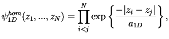
For infinitely strong particle interactions (
![]() ),
Girardeau shows [Gir60], using the equivalence between the 1D
),
Girardeau shows [Gir60], using the equivalence between the 1D
![]() -function potential and a ``1D hard-point potential'', that the energy
spectrum of the 1D Bose gas coincides with that of
-function potential and a ``1D hard-point potential'', that the energy
spectrum of the 1D Bose gas coincides with that of ![]() non-interacting
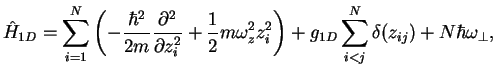
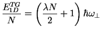
spin-polarized fermions. The lowest eigenenergy per particle of the trapped 1D Bose
gas, Eq. 4.21, is, in the TG limit, given by4.1
non-interacting
spin-polarized fermions. The lowest eigenenergy per particle of the trapped 1D Bose
gas, Eq. 4.21, is, in the TG limit, given by4.1
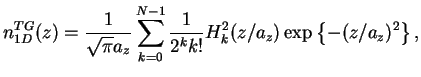
The corresponding gas density is given by the sum of squares of single-particle
wave functions
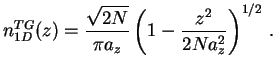
The above result cannot reproduce the oscillatory behavior of the exact density, Eq. 4.23, but it does describe the overall behavior properly (see Sec. 4.5).
To characterize the inhomogeneous 1D Bose gas further, we consider the
many-body Hamiltonian of the homogeneous 1D Bose gas,
By introducing the energy shift
![]() , our classification of
gas-like states and cluster-like bound states introduced after Eq. 4.21
remains valid. For positive
, our classification of
gas-like states and cluster-like bound states introduced after Eq. 4.21
remains valid. For positive ![]() ,
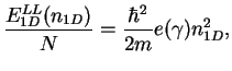
, ![]() corresponds to the
Lieb-Liniger (LL) Hamiltonian. The gas-like states of the LL Hamiltonian, including
its thermodynamic properties, have been studied in detail [LL63,Lie63,YY69]. The energy
per particle of the lowest-lying gas-like state, the ground state of the system, is
given by
corresponds to the
Lieb-Liniger (LL) Hamiltonian. The gas-like states of the LL Hamiltonian, including
its thermodynamic properties, have been studied in detail [LL63,Lie63,YY69]. The energy
per particle of the lowest-lying gas-like state, the ground state of the system, is
given by
We use the known properties of the LL Hamiltonian to determine properties of the
corresponding inhomogeneous system, Eq. 4.19, within the LDA. This
approximation provides a correct description of the trapped gas if the size of the
atomic cloud is much larger than the characteristic length scale ![]() of the
confinement in the longitudinal direction [DLO01]. Specifically, consider
the local equilibrium condition,
of the
confinement in the longitudinal direction [DLO01]. Specifically, consider
the local equilibrium condition,
The chemical potential ![]() , Eq. 4.27, can be calculated using
Eq. 4.28 together with the normalization of the density,
, Eq. 4.27, can be calculated using
Eq. 4.28 together with the normalization of the density,
![]() . Integrating the chemical potential
. Integrating the chemical potential
![]() then determines the energy of the lowest-lying gas-like state of the
inhomogeneous
then determines the energy of the lowest-lying gas-like state of the
inhomogeneous ![]() -particle system within the LDA. The LDA treatment is
computationally less demanding than solving the many-body Schrödinger equation,
Eq. 4.21, using MC techniques. By comparing with our full 1D many-body
results we establish the accuracy of the LDA (see Sec. 4.4.1).
-particle system within the LDA. The LDA treatment is
computationally less demanding than solving the many-body Schrödinger equation,
Eq. 4.21, using MC techniques. By comparing with our full 1D many-body
results we establish the accuracy of the LDA (see Sec. 4.4.1).
For negative ![]() , the Hamiltonian given in Eq. 4.25 supports
cluster-like bound states. The ground state energy and eigenfunction of the system
are [McG64]
, the Hamiltonian given in Eq. 4.25 supports
cluster-like bound states. The ground state energy and eigenfunction of the system
are [McG64]
The above discussion implies that the lowest-lying gas-like state of the 1D
Hamiltonian with confinement, Eq. 4.19 with negative ![]() ,
corresponds to a highly-excited state. For dilute 1D systems with negative
,
corresponds to a highly-excited state. For dilute 1D systems with negative
![]() , the nodal surface of this excited state can be well approximated by the
following nodal surface:
, the nodal surface of this excited state can be well approximated by the
following nodal surface: ![]() for
for ![]() , where
, where
![]() and
and ![]() . As in the two-body case, the many-body energy can then be calculated
approximately by restricting the configuration space to regions where the wave
function is positive. This corresponds to treating a gas of hard-rods of size
. As in the two-body case, the many-body energy can then be calculated
approximately by restricting the configuration space to regions where the wave
function is positive. This corresponds to treating a gas of hard-rods of size
![]() . In the low density limit, we expect that the lowest-lying gas-like state
of the 1D many-body Hamiltonian with
. In the low density limit, we expect that the lowest-lying gas-like state
of the 1D many-body Hamiltonian with ![]() is well described by a system of
hard-rods of size
is well described by a system of
hard-rods of size ![]() .
.
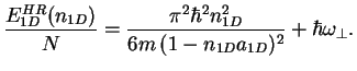
In addition to treating the full 1D many-body Hamiltonian, we treat the
inhomogeneous system with negative ![]() within the LDA. The equation of state
of the uniform hard-rod gas with density
within the LDA. The equation of state
of the uniform hard-rod gas with density ![]() is given
by (1.103) [Gir60]:
is given
by (1.103) [Gir60]:
We use this energy in the LDA treatment (see Eqs. 4.26 through
4.28 with ![]() replaced by
replaced by ![]() ). The hard-rod
equation of state treated within the LDA provides a good description when
). The hard-rod
equation of state treated within the LDA provides a good description when ![]() is negative, but
is negative, but ![]() not too small (see Secs. 4.4.1 and
4.5). To gain more insight, we determine the expansion for inhomogeneous
systems with
not too small (see Secs. 4.4.1 and
4.5). To gain more insight, we determine the expansion for inhomogeneous
systems with
![]() using the equation of state for the homogeneous
hard-rod gas,
using the equation of state for the homogeneous
hard-rod gas,
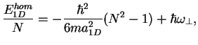
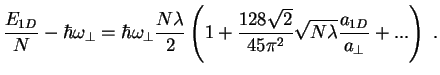
The first term corresponds to the energy per particle in the TG regime (see
Eq. 4.22), the other terms can be considered as small corrections to the TG
energy. In the unitary limit, that is, for
![]() , expression
(4.32) becomes independent of
, expression
(4.32) becomes independent of ![]() , and depends only on
, and depends only on
![]() . Similarly, the linear density in the center of the cloud,
. Similarly, the linear density in the center of the cloud, ![]() , is to
lowest order given by the TG result,
, is to
lowest order given by the TG result,
![]() (see Eq. 4.24). Section 4.5 shows that the TG density
provides a good description of inhomogeneous 1D Bose gases over a fairly large range
of negative
(see Eq. 4.24). Section 4.5 shows that the TG density
provides a good description of inhomogeneous 1D Bose gases over a fairly large range
of negative ![]() .
.
![$\displaystyle \hat H_{3D}= \sum_{i=1}^N \left[-\frac{\hbar^2}{2m}\Delta_i
+ \fr...
...a_\perp^2 \rho_i^2
+ \omega_z^2 z_i^2 \right) \right] + \sum_{i<j}^N V(r_{ij}),$](img1221.gif)
![$\displaystyle \mu(N)= \hbar \omega_\perp + \mu_{local}[n_{1D}(z)]+\frac{1}{2}m \omega_z^2 z^2,$](img1240.gif)
![$\displaystyle \mu_{local}(n_{1D}) = \frac{\partial\left[
n_{1D} E_{1D}^{LL}(n_{1D})/N
\right]}{\partial n_{1D}}.$](img1242.gif)